Obtaining prediction bands for regression model

Question

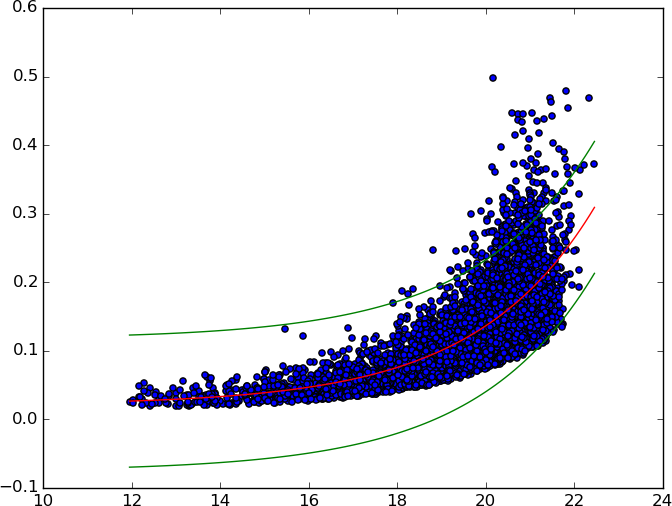
I'm trying to generate prediction bands for an exponential fit to some 2-dimensional data (available here).

The data (blue points), best fit found by scipy.optimize.curve_fit (red curve), and lower & upper 95% prediction bands (green curves) can be seen in the image below.

I'd love some confirmation that the code is actually doing things correctly and I haven't missed some step or simply used the wrong statistical tools.

The references I used are basically this post, and this video, both adapted to work with a general function, rather than being hardcoded to work with a linear function of the form \$y = a*x+b\$.

import numpy as np
import matplotlib.pyplot as plt
from scipy.optimize import curve_fit
from scipy import stats


def make_plot(x, xd, yd, popt, upb, lpb):
    # Plot data.
    plt.scatter(xd, yd)
    # Plot best fit curve.
    plt.plot(x, func(x, *popt), c='r')
    # Prediction band (upper)
    plt.plot(x, upb, c='g')
    # Prediction band (lower)
    plt.plot(x, lpb, c='g')
    plt.show()


def func(x, a, b, c):
    '''Exponential 3-param function.'''
    return a * np.exp(b * x) + c


def predband(x, xd, yd, f_vars, conf=0.95):
    """
    Code adapted from Rodrigo Nemmen's post:
    http://astropython.blogspot.com.ar/2011/12/calculating-prediction-band-
    of-linear.html

    Calculates the prediction band of the regression model at the
    desired confidence level.

    Clarification of the difference between confidence and prediction bands:

    "The prediction bands are further from the best-fit line than the
    confidence bands, a lot further if you have many data points. The 95%
    prediction band is the area in which you expect 95% of all data points
    to fall. In contrast, the 95% confidence band is the area that has a
    95% chance of containing the true regression line."
    (from http://www.graphpad.com/guides/prism/6/curve-fitting/index.htm?
    reg_graphing_tips_linear_regressio.htm)

    Arguments:
    - x: array with x values to calculate the confidence band.
    - xd, yd: data arrays.
    - a, b, c: linear fit parameters.
    - conf: desired confidence level, by default 0.95 (2 sigma)

    References:
    1. http://www.JerryDallal.com/LHSP/slr.htm, Introduction to Simple Linear
    Regression, Gerard E. Dallal, Ph.D.
    """

    alpha = 1. - conf    # Significance
    N = xd.size          # data sample size
    var_n = len(f_vars)  # Number of variables used by the fitted function.

    # Quantile of Student's t distribution for p=(1 - alpha/2)
    q = stats.t.ppf(1. - alpha / 2., N - var_n)

    # Std. deviation of an individual measurement (Bevington, eq. 6.15)
    se = np.sqrt(1. / (N - var_n) * np.sum((yd - func(xd, *f_vars)) ** 2))

    # Auxiliary definitions
    sx = (x - xd.mean()) ** 2
    sxd = np.sum((xd - xd.mean()) ** 2)

    # Predicted values (best-fit model)
    yp = func(x, *f_vars)
    # Prediction band
    dy = q * se * np.sqrt(1. + (1. / N) + (sx / sxd))

    # Upper & lower prediction bands.
    lpb, upb = yp - dy, yp + dy

    return lpb, upb


# Read data from file.
xd, yd = np.loadtxt('exponential_data.dat', unpack=True)

# Find best fit of data with 3-parameters exponential function.
popt, pcov = curve_fit(func, xd, yd)

# Generate equi-spaced x values.
x = np.linspace(xd.min(), xd.max(), 100)

# Call function to generate lower an upper prediction bands.
lpb, upb = predband(x, xd, yd, popt, conf=0.95)

# Plot.
make_plot(x, xd, yd, popt, upb, lpb)

Answer 1

There is a nice discussion about confidence/prediction bands in the documentation for the excellent kmpfit module. You need to include the convariance matrix from the fit in the calculation of the bands, which I don't see in your code. There is an example in the link that walks through it.

Here is their implementation:

def confpred_band(x, dfdp, prob, fitobj, f, prediction, abswei=False, err=None):
   #----------------------------------------------------------
   # Return values for a confidence or a prediction band.
   # See documentation for methods confidence_band and 
   # prediction_band
   #----------------------------------------------------------   
   from scipy.stats import t
   # Given the confidence or prediction probability prob = 1-alpha
   # we derive alpha = 1 - prob 
   alpha = 1 - prob
   prb = 1.0 - alpha/2
   tval = t.ppf(prb, fitobj.dof)

   C = fitobj.covar
   n = len(fitobj.params)              # Number of parameters from covariance matrix
   p = fitobj.params
   N = len(x)
   if abswei:
      covscale = 1.0  # Do not apply correction with red. chi^2
   else:
      covscale = fitobj.rchi2_min
   df2 = numpy.zeros(N)
   for j in range(n):
      for k in range(n):
         df2 += dfdp[j]*dfdp[k]*C[j,k]
   if prediction:
      df = numpy.sqrt(err*err+covscale*df2)
   else:
      df = numpy.sqrt(covscale*df2)
   y = f(p, x)
   delta = tval * df   
   upperband = y + delta
   lowerband = y - delta 
   return y, upperband, lowerband