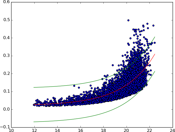
I'm trying to generate prediction bands for an exponential fit to some 2-dimensional data (available here).

The data (blue points), best fit found by scipy.optimize.curve_fit (red curve), and lower & upper 95% prediction bands (green curves) can be seen in the image below.

(the MWE is at the bottom of the question)

I'd love some confirmation that the code is actually doing things correctly and I haven't missed some step or simply used the wrong statistical tools.

The references I used are basically this post, and this video, both adapted to work with a general function, rather than being hardcoded to work with a linear function of the form y=a*x+b.

Any suggested improvements on the code will also be appreciated.

MWE

import numpy as np
import matplotlib.pyplot as plt
from scipy.optimize import curve_fit
from scipy import stats


def make_plot(x, xd, yd, popt, upb, lpb):
    # Plot data.
    plt.scatter(xd, yd)
    # Plot best fit curve.
    plt.plot(x, func(x, *popt), c='r')
    # Prediction band (upper)
    plt.plot(x, upb, c='g')
    # Prediction band (lower)
    plt.plot(x, lpb, c='g')
    plt.show()


def func(x, a, b, c):
    '''Exponential 3-param function.'''
    return a * np.exp(b * x) + c


def predband(x, xd, yd, f_vars, conf=0.95):
    """
    Code adapted from Rodrigo Nemmen's post:
    http://astropython.blogspot.com.ar/2011/12/calculating-prediction-band-
    of-linear.html

    Calculates the prediction band of the regression model at the
    desired confidence level.

    Clarification of the difference between confidence and prediction bands:

    "The prediction bands are further from the best-fit line than the
    confidence bands, a lot further if you have many data points. The 95%
    prediction band is the area in which you expect 95% of all data points
    to fall. In contrast, the 95% confidence band is the area that has a
    95% chance of containing the true regression line."
    (from http://www.graphpad.com/guides/prism/6/curve-fitting/index.htm?
    reg_graphing_tips_linear_regressio.htm)

    Arguments:
    - x: array with x values to calculate the confidence band.
    - xd, yd: data arrays.
    - a, b, c: linear fit parameters.
    - conf: desired confidence level, by default 0.95 (2 sigma)

    References:
    1. http://www.JerryDallal.com/LHSP/slr.htm, Introduction to Simple Linear
    Regression, Gerard E. Dallal, Ph.D.
    """

    alpha = 1. - conf    # Significance
    N = xd.size          # data sample size
    var_n = len(f_vars)  # Number of variables used by the fitted function.

    # Quantile of Student's t distribution for p=(1 - alpha/2)
    q = stats.t.ppf(1. - alpha / 2., N - var_n)

    # Std. deviation of an individual measurement (Bevington, eq. 6.15)
    se = np.sqrt(1. / (N - var_n) * np.sum((yd - func(xd, *f_vars)) ** 2))

    # Auxiliary definitions
    sx = (x - xd.mean()) ** 2
    sxd = np.sum((xd - xd.mean()) ** 2)

    # Predicted values (best-fit model)
    yp = func(x, *f_vars)
    # Prediction band
    dy = q * se * np.sqrt(1. + (1. / N) + (sx / sxd))

    # Upper & lower prediction bands.
    lpb, upb = yp - dy, yp + dy

    return lpb, upb


# Read data from file.
xd, yd = np.loadtxt('exponential_data.dat', unpack=True)

# Find best fit of data with 3-parameters exponential function.
popt, pcov = curve_fit(func, xd, yd)

# Generate equi-spaced x values.
x = np.linspace(xd.min(), xd.max(), 100)

# Call function to generate lower an upper prediction bands.
lpb, upb = predband(x, xd, yd, popt, conf=0.95)

# Plot.
make_plot(x, xd, yd, popt, upb, lpb)