3
\$\begingroup\$

I am loading a bunch of arrays and putting them into a single array. The loading of the data is negligible, but putting it into combinedArray takes significant time (as in this code).

import time
import numpy as np
start_time = time.time()

   st,en = 0,0
   combinedArray = np.empty(shape = (30000*30000))
   #Get the array that each process wrote to
   for i in range(10):
       #load the array
       #ex loading 
       X_np = np.empty(shape = (30000*30000)/10)
       st = en
       en += np.shape(X_np[:])[0]
       #add to the array list
       combinedArray[st:en] = X_np[:]

   print("Array Calc:",time.time()-start_time)  

What I have found is often someone talking about not using append, so I tried with creating the array first, but just moving it is time consuming. Any advice on how to optimize this is appreciated.

\$\endgroup\$

2 Answers 2

2
\$\begingroup\$

I performed some timings of the solutions presented by @AustinHastings in his answer on my machine at work (Linux 64bit, Intel Core i7-2600, 16GB RAM, Anaconda Python 3, ).

The timing function was slightly modified to use repetitions get more accurate results as well as to easier get the timings for visual display.

def time_func(f, shape=1000, n_reps=10):
    global COMBINED_SHAPE
    COMBINED_SHAPE = shape
    start_time = timeit.default_timer()
    for _ in range(n_reps):
        ca = f()
        assert np.shape(ca)[0] == COMBINED_SHAPE
    average_time = (timeit.default_timer() - start_time) / n_reps
    print(f"Time for {f.__name__}: "
          f"{average_time * 1000:.6f} ms")
    return average_time

# the functions go here

def perform_benchmark(*shapes):
    results = np.zeros((len(shapes), 5))
    for i, shape in enumerate(shapes):
        print(f"shape: {shape}")
        print(f"array size: {shape * 8 / 1024**3:.3f} GB")
        results[i, 0] = time_func(orig, shape=shape)
        results[i, 1] = time_func(concat, shape=shape)
        results[i, 2] = time_func(block, shape=shape)
        results[i, 3] = time_func(stack_ravel, shape=shape)
        results[i, 4] = time_func(stack_flatten, shape=shape)

    plt.figure()
    plt.plot(shapes, results, marker="o")
    plt.xlim((shapes[0], shapes[-1]))
    plt.grid(ls="--")
    plt.legend(["orig", "concat", "block", "stack_ravel", "stack_flatten"])

    plt.figure()
    plt.loglog(shapes, results, marker="o")
    plt.xlim((shapes[0], shapes[-1]))
    plt.grid(ls="--")
    plt.legend(["orig", "concat", "block", "stack_ravel", "stack_flatten"])

    plt.show()


if __name__ == '__main__':
    perform_benchmark(
           100000,    300000,    500000,
          1000000,   3000000,   5000000,
         10000000,  30000000,  50000000,
        100000000, 300000000
    )

The array size of \$500 \times 10^6\$ elements which would have come next was to big to fit in RAM and lead to excessive swapping (your original would be at \$ 900 \times 10^6 \$).

When looking at the linear plot you will see no difference between the solutions on all but stack_flatten which consistently takes about twice the time of the other solutions.
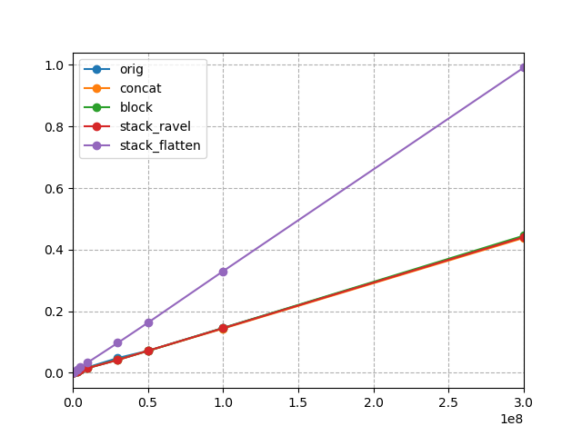
double linear plot

In an loglog graph you can see this as an approximately constant offset between stack_flatten and the other solutions.
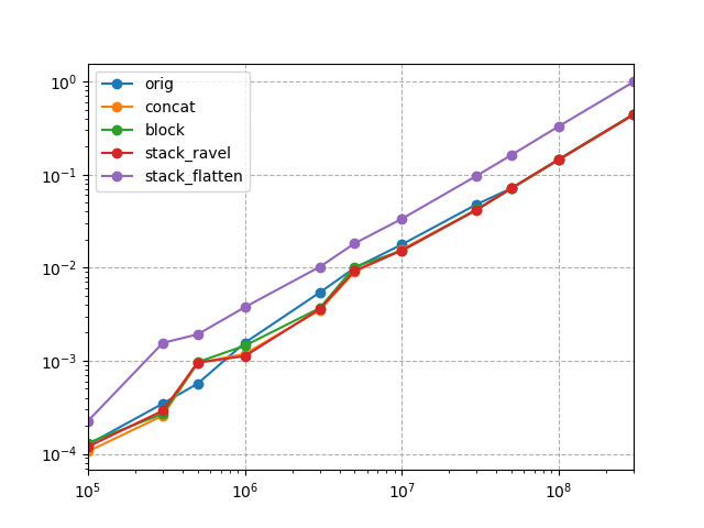
enter image description here

These findings seem to be consistent with what Austin Hastings presented in his answer.

\$\endgroup\$
2
\$\begingroup\$

I tried some alternative approaches, and got this result:

Time for orig: 0.15900921821594238
Time for concat: 0.18401050567626953
Time for block: 0.16700983047485352
Time for stack_ravel: 0.1760098934173584
Time for stack_flatten: 0.32501864433288574

It's worth pointing out that I'm on a 32-bit machine with not enough RAM to hang with you. So I used smaller arrays. You'll want to correct the code and try for yourself. Also, my validation is really minimal, so you should probably improve that as well.

import time
import numpy as np

COMBINED_SHAPE = (3_000 * 3_000)

def time_func(f):
    start_time = time.time()
    ca = f()
    assert np.shape(ca)[0] == COMBINED_SHAPE
    print(f"Time for {f.__name__}:", time.time() - start_time)

def load_partial():
    partial = np.empty(shape=(COMBINED_SHAPE // 10))
    return partial

def orig():
    st, en = 0, 0
    combined_array = np.empty(shape=COMBINED_SHAPE)

    for i in range(10):
        X_np = load_partial()
        st = en
        en += np.shape(X_np[:])[0]
        combined_array[st:en] = X_np[:]

    return combined_array

def concat():
    ca = np.concatenate([load_partial() for _ in range(10)])
    return ca

def block():
    ca = np.block([load_partial() for _ in range(10)])
    return ca

def stack_ravel():
    ca = np.stack([load_partial() for _ in range(10)])
    ca = np.ravel(ca)
    return ca

def stack_flatten():
    ca = np.stack([load_partial() for _ in range(10)]).flatten()
    return ca


if __name__ == '__main__':
    time_func(orig)
    time_func(concat)
    time_func(block)
    time_func(stack_ravel)
    time_func(stack_flatten)
\$\endgroup\$
2
  • \$\begingroup\$ Just to make sure I am understanding, the time just shows the original is faster? \$\endgroup\$ Commented May 25, 2019 at 12:45
  • \$\begingroup\$ Yes, it shows the original is faster on my horribly old machine. I'd strongly suggest running the timing framework on the actual hardware you intend to use, since it's very likely to have different performance characteristics. \$\endgroup\$
    – aghast
    Commented May 25, 2019 at 15:05

Your Answer

By clicking “Post Your Answer”, you agree to our terms of service and acknowledge you have read our privacy policy.

Not the answer you're looking for? Browse other questions tagged or ask your own question.