Turn on Option Explicit. From the menu at the top Tools>Option>Editor tab>Code Settings group>Require Variable Declaration check box. Make sure that is checked. This mandates that you use Dim foo as Bar before you can use any variables and will save you needless headaches. Why? myRange is not declared anywhere and a simple typo can mean a half hour or more debugging to find that typo. This will add Option Explicit automatically to any new code modules. It's on you however to add it any existing code modules.
Multiple variables declared on one line. Dim i, iLastSource, iRowTarget, count As Long only count is declared as a Long type. The rest are Variant. Likewise for Dim wsSource, wsTarget As Worksheet only wsTarget has the type of Worksheet, wsSource if of type Variant. Fix this by declaring each variable on its own line. Also declare them just before you use them. This makes refactoring easier and avoids unused variables.
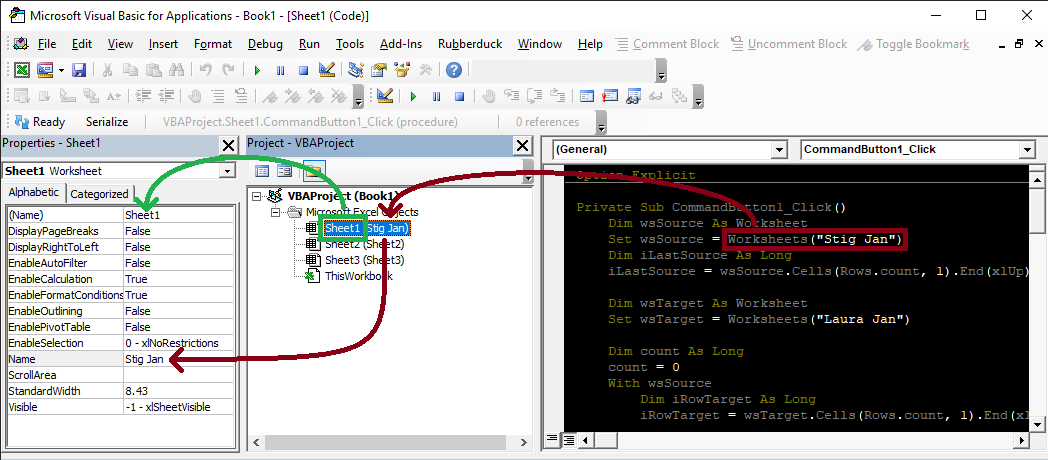
Your Stig Jan worksheet isn't created in the click event which means it's available at design time. Reference that worksheet by using the Worksheet.CodeName property. In the VBIDE under View>Properties Window (Hotkey: F4). Rename the CodeName, shown in properties window as (Name) property, to a descriptive name. I've rename it to StigJan.

Then you can reference that worksheet directly. This way if the name of the worksheet changes your code won't break.

Hungarian notation isn't needed. Because you have your variables declared with a type As Worksheet you don't need the ws prefix. Place your cursor on a variable name and from the menu at the top Edit>Quick Info (Hotkey: Ctrl+I) you can display the variables type.

Your For ... Next statement logic can be simplified. You're looping with the counter i but within that loop setting a cell variable. This is a candidate for a For Each ... Next statement.
For i = 36 To iLastSource
    Dim cell As Worksheet
    Set cell = .Cells(i, 4)
Becomes the code below. This clarifies the intent that you're looping through each cell in the area.
Dim checkArea As Range
Set checkArea = source.Range(source.Cells(36, 4), source.Cells(iLastSource, 4))
Dim checkCell As Range
For Each checkCell In checkArea
Once you've done that the next step is to consolidate the if checks. cell.Font.Bold = False can be rewritten as Not cell.Font.Bold. Combine that into a single check with the value check of the cell below it.
If cell.Font.Bold = False Then
    If cell.Value = "Fælles" Then
Becomes
If Not checkCell.Font.Bold And checkCell.Value = "Fælles" Then
The body within the If statement can then be reviewed. The parts that change are "STIGS ", "A", "H", "D".
cell.Offset(, 1).Value = "STIGS " & cell.Offset(, 1).Value
wsTarget.Range("A" & iRowTarget & ":H" & iRowTarget).Value = .Range("A" & i & ":H" & i).Value
wsTarget.Range("D" & iRowTarget).ClearContents
iRowTarget = iRowTarget + 1
count = count + 1
We extract that into its own dedicated Sub and supply the arguments that let it requires. The parameters targetRow, and copiedRowCount have the ByRef modifier because we want any changes to be reflected in the calling member after this Sub finishes.
Private Sub UpdateOffsetCellAndClearContents(ByVal checkCell As Range, _
                                                ByVal sourceWorksheet As Worksheet, _
                                                ByVal targetWorksheet As Worksheet, _
                                                ByRef targetRow As Long, _
                                                ByVal leftTargetColumn As Variant, _
                                                ByVal rightTargetColumn As Variant, _
                                                ByVal columnOfCellToClear As Variant, _
                                                ByVal offsetPrefixValue As String, _
                                                ByRef copiedRowCount As Long)
    checkCell.Offset(ColumnOffset:=1).Value = offsetPrefixValue & " " & checkCell.Offset(ColumnOffset:=1).Value

    Dim destinationArea As Range
    Set destinationArea = targetWorksheet.Range(targetWorksheet.Cells(targetRow, leftTargetColumn), targetWorksheet.Cells(targetRow, rightTargetColumn))
    Dim sourceArea As Range
    Set sourceArea = sourceWorksheet.Range(sourceWorksheet.Cells(checkCell.Row, leftTargetColumn), sourceWorksheet.Cells(checkCell.Row, rightTargetColumn))
    destinationArea.Value2 = sourceArea.Value2

    targetWorksheet.Cells(targetRow, columnOfCellToClear).ClearContents

    targetRow = targetRow + 1
    copiedRowCount = copiedRowCount + 1
End Sub
The call sites where this is used.
UpdateOffsetCellAndClearContents checkCell, source, target, targetRow, "A", "H", "D", "STIGS ", count
...
UpdateOffsetCellAndClearContents checkCell, source, target, targetRow, "A", "H", "D", "STIG ", count
...
UpdateOffsetCellAndClearContents checkCell, source, target, targetRow, "K", "R", "N", "STIGS ", count
...
UpdateOffsetCellAndClearContents checkCell, source, target, targetRow, "K", "R", "N", "STIG ", count
Now if/when you need to make an update to the logic you change it within the Sub and all sites where it's called are now updated.
Instead of If cell.Value = "Fælles" Or cell.Value = "Lagt Ud" Then to bold the font or If myCell Like "*STIG*" Then to color a cells interior use conditional formatting. That way you set it for the entire range and it will automatically be applied whenever the cell changes. For their respective parts I came up with the below for bolding and
Private Sub AddBoldConditionalFormattingTo(ByVal formatArea As Range, ParamArray values())
    If formatArea.FormatConditions.count > 0 Then
        formatArea.FormatConditions.Delete
    End If

    Dim topLeftAddress As String
    topLeftAddress = formatArea.Cells(1, 1).Address(False, False)
    Dim orArguments As String
    orArguments = topLeftAddress & "=""" & Join(values, """," & topLeftAddress & "=""") & """"
    Dim formulaForTopLeftCell As String
    formulaForTopLeftCell = "=OR(" & orArguments & ")"

    Dim addedCondition As FormatCondition
    Set addedCondition = formatArea.FormatConditions.Add(XlFormatConditionType.xlExpression, Formula1:=formulaForTopLeftCell)
    addedCondition.Font.Bold = True
End Sub

Private Sub AddInteriorColorConditionalFormattingTo(ByVal formatArea As Range, ByVal interiorColor As Long, ByVal valueToSearchFor As String)
    If formatArea.FormatConditions.count > 0 Then
        formatArea.FormatConditions.Delete
    End If

    Dim formulaForTopLeftCell As String
    formulaForTopLeftCell = "=NOT(ISERROR(SEARCH(""" & "STIG" & """," & formatArea.Cells(1, 1).Address(False, False) & ")))"

    Dim addedCondition As FormatCondition
    Set addedCondition = formatArea.FormatConditions.Add(XlFormatConditionType.xlExpression, Formula1:=formulaForTopLeftCell, TextOperator:=XlContainsOperator.xlContains)
    addedCondition.Interior.Color = interiorColor
End Sub
Their respective call sites as below
AddBoldConditionalFormattingTo checkArea, "Fælles", "Lagt Ud"
and
AddInteriorColorConditionalFormattingTo target.Range("A36:S1000"), "STIG", RGB(255, 220, 220)
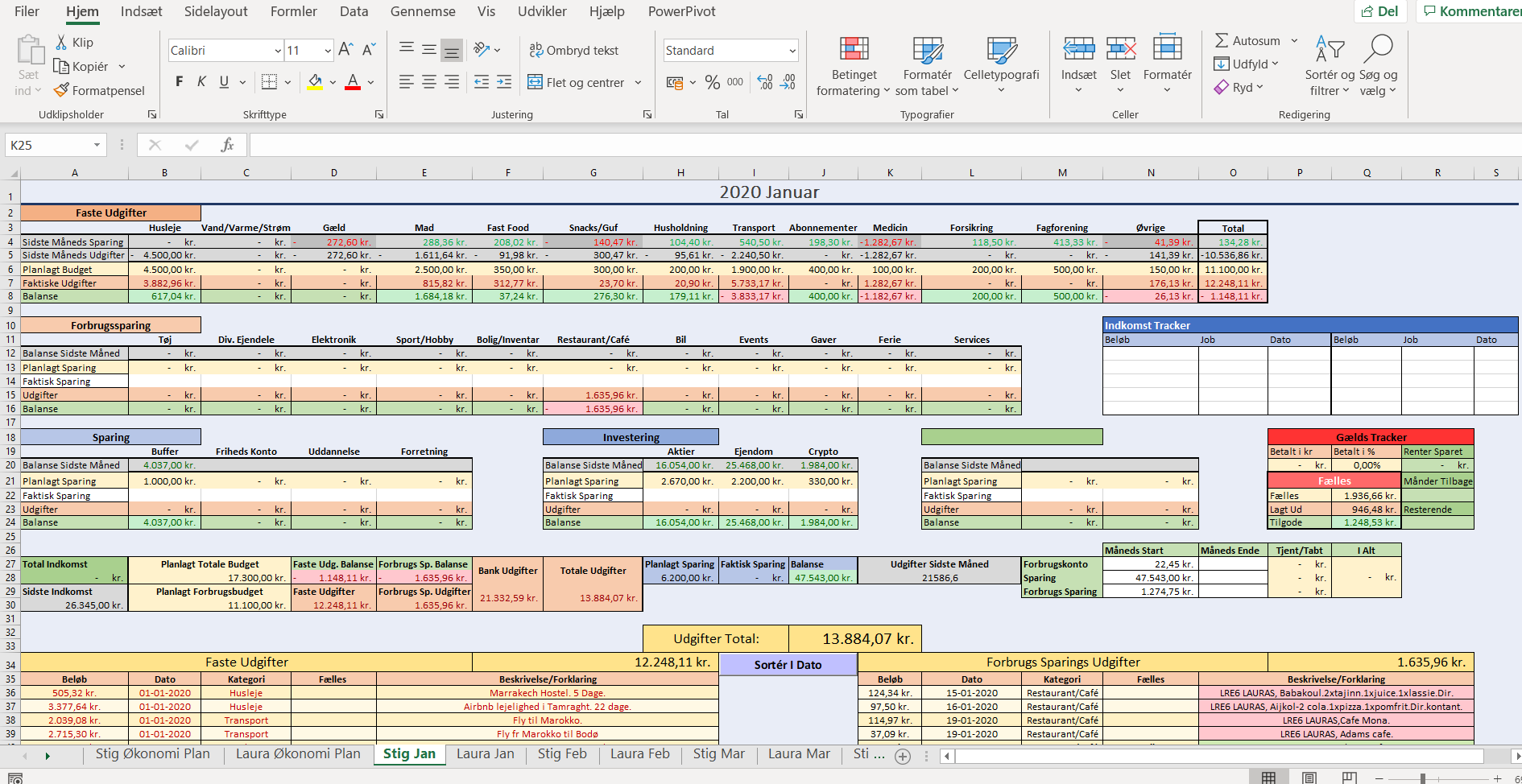
Static cell ranges. Range("K76") will break whenever a row above or column to the left is inserted/deleted, as will Range("A36:S1000"). Make these named ranges and reference them through the named ranges because named ranges don't break with insertions/deletions. I have no clue what these cells represent and can't begin to offer a suggestion.
Magic numbers. 36 has what significance? It's in the code for some reason. Why is it there? Use a name to describe why its there and/or its siginificance. If this number will never ever change convert it to a Const statement with a descriptive name like Const StartRow As Long = 36. If it may vary at run-time determine its value and assign it
dim startRow As Long
startRow = source.Cells(1,4).End(xlDown).Row + 1
The refactored code below reflect these changes
Option Explicit

Private Sub CommandButton1_Click()
    Dim source As Worksheet
    Set source = StigJan
    Dim lastSourceRow As Long
    lastSourceRow = source.Cells(Rows.count, 1).End(xlUp).Row

    Dim target As Worksheet
    Set target = LauraJan

    Dim targetRow As Long
    targetRow = target.Cells(Rows.count, 1).End(xlUp).Row + 1

    Const StartRow As Long = 36

    Dim count As Long
    Dim checkArea As Range
    Set checkArea = source.Range(source.Cells(StartRow, 4), source.Cells(lastSourceRow, 4))
    Dim checkCell As Range
    For Each checkCell In checkArea
        If Not checkCell.Font.Bold And checkCell.Value = "Fælles" Then
            UpdateOffsetCellAndClearContents checkCell, source, target, targetRow, "A", "H", "D", "STIGS ", count
        End If

        If Not checkCell.Font.Bold And checkCell.Value = "Lagt Ud" Then
            UpdateOffsetCellAndClearContents checkCell, source, target, targetRow, "A", "H", "D", "STIG ", count
        End If
    Next
    AddBoldConditionalFormattingTo checkArea, "Fælles", "Lagt Ud"

    targetRow = target.Range("K76").End(xlUp).Row + 1
    Set checkArea = source.Range(source.Cells(StartRow, 14), source.Cells(lastSourceRow, 14))
    For Each checkCell In checkArea
        If Not checkCell.Font.Bold And checkCell.Value = "Fælles" Then
            UpdateOffsetCellAndClearContents checkCell, source, target, targetRow, "K", "R", "N", "STIGS ", count
        End If

        If Not checkCell.Font.Bold And checkCell.Value = "Lagt Ud" Then
            UpdateOffsetCellAndClearContents checkCell, source, target, targetRow, "K", "R", "N", "STIG ", count
        End If
    Next
    AddBoldConditionalFormattingTo checkArea, "Fælles", "Lagt Ud"

    AddInteriorColorConditionalFormattingTo target.Range("AdequatelyNamedArea"), "STIG", RGB(255, 220, 220)

    MsgBox "Done : " & count & " rows copied"
End Sub

Private Sub UpdateOffsetCellAndClearContents(ByVal checkCell As Range, _
                                                ByVal sourceWorksheet As Worksheet, _
                                                ByVal targetWorksheet As Worksheet, _
                                                ByRef targetRow As Long, _
                                                ByVal leftTargetColumn As Variant, _
                                                ByVal rightTargetColumn As Variant, _
                                                ByVal columnOfCellToClear As Variant, _
                                                ByVal offsetPrefixValue As String, _
                                                ByRef copiedRowCount As Long)
    checkCell.Offset(ColumnOffset:=1).Value = offsetPrefixValue & " " & checkCell.Offset(ColumnOffset:=1).Value

    Dim destinationArea As Range
    Set destinationArea = targetWorksheet.Range(targetWorksheet.Cells(targetRow, leftTargetColumn), targetWorksheet.Cells(targetRow, rightTargetColumn))
    Dim sourceArea As Range
    Set sourceArea = sourceWorksheet.Range(sourceWorksheet.Cells(checkCell.Row, leftTargetColumn), sourceWorksheet.Cells(checkCell.Row, rightTargetColumn))
    destinationArea.Value2 = sourceArea.Value2

    targetWorksheet.Cells(targetRow, columnOfCellToClear).ClearContents

    targetRow = targetRow + 1
    copiedRowCount = copiedRowCount + 1
End Sub

Private Sub AddBoldConditionalFormattingTo(ByVal formatArea As Range, ParamArray values())
    If formatArea.FormatConditions.count > 0 Then
        formatArea.FormatConditions.Delete
    End If

    Dim topLeftAddress As String
    topLeftAddress = formatArea.Cells(1, 1).Address(False, False)
    Dim orArguments As String
    orArguments = topLeftAddress & "=""" & Join(values, """," & topLeftAddress & "=""") & """"
    Dim formulaForTopLeftCell As String
    formulaForTopLeftCell = "=OR(" & orArguments & ")"

    Dim addedCondition As FormatCondition
    Set addedCondition = formatArea.FormatConditions.Add(XlFormatConditionType.xlExpression, Formula1:=formulaForTopLeftCell)
    addedCondition.Font.Bold = True
End Sub

Private Sub AddInteriorColorConditionalFormattingTo(ByVal formatArea As Range, ByVal interiorColor As Long, ByVal valueToSearchFor As String)
    If formatArea.FormatConditions.count > 0 Then
        formatArea.FormatConditions.Delete
    End If

    Dim formulaForTopLeftCell As String
    formulaForTopLeftCell = "=NOT(ISERROR(SEARCH(""" & valueToSearchFor & """," & formatArea.Cells(1, 1).Address(False, False) & ")))"

    Dim addedCondition As FormatCondition
    Set addedCondition = formatArea.FormatConditions.Add(XlFormatConditionType.xlExpression, Formula1:=formulaForTopLeftCell, TextOperator:=XlContainsOperator.xlContains)
    addedCondition.Interior.Color = interiorColor
End Sub


